Collaborative Multi-Robot
Non-Prehensile Manipulation via Flow-Matching Co-Generation
Yorai Shaoul, Zhe Chen*, Naveed Gul Mohamed*,
Federico Pecora, Maxim Likhachev, and Jiaoyang Li.


Our Goal
Explore multi-robot collaboration.
Collaboration is:
Collaboration
Robots work together, and depend on each other, to complete a global task.
Collaboration is not:
Coordination
Robots execute learned behaviors in a shared
environment to complete private tasks.
The Collaborative Manipulation Problem
Given
- a set of \(N\) robots \(\mathcal{R} := \{\mathcal{R}_i\}_{i=1}^N\),
- observations of movable objects
\(\mathcal{O} := \{\mathcal{O}_j\}\), \(\mathcal{I}(\mathcal{O}_j) \in \mathbb{R}^{W\times W}\), - Poses and shapes of obstacles,
- Target poses for all objects.
We want to
Compute a set of motions \(\Tau := \{\tau^i\}_{i=1}^N \) such that, upon execution, all objects arrive at their goals.
The online problem
Compute short-horizon motions \(\Tau := \{\tau^i\}_{i=1}^N \), execute them, and repeat. Eventually, the objects must arrive at their goals.
Planning and Learning For Collaboration
Plan motions
to contact points
Learn physical
interactions
Plan motions
for objects
Planning and Learning For Collaboration
We interleave plannning and learning in a generative collaboration framework \(\text{GC}\scriptsize{\text{O}}\).
Learn what we "must," and plan what we can.
Difficult to model
Available geometric models
Agenda
- We'll start by looking at learning manipulation interactions,
- Continue to our multi-robot planning algorithm \(\text{G}\scriptsize{\text{SPI}}\)
Plan motions
to contact points
Learn physical
interactions
Plan motions
for objects
Planning and Learning For Collaboration
Learning Multi-Robot Manipulation
We seek to learn two things:
- Manipulation trajectories
- Contact points
In this work, we do so jointly with imitation learning.
Learning Multi-Robot Manipulation
We seek to learn two things:
- Manipulation trajectories
- Contact points
Learning Multi-Robot Manipulation
We seek to learn two things:
- Manipulation trajectories
- Contact points
Learning Multi-Robot Manipulation
We seek to learn two things:
- Manipulation trajectories
- Contact points
Learning Multi-Robot Manipulation
We seek to learn two things:
- Manipulation trajectories
- Contact points
Learning Multi-Robot Manipulation
Many manipulation trajectories and contact points
combinations are valid, but not all are useful.
Learning Multi-Robot Manipulation
Many manipulation trajectories and contact points
combinations are valid, but not all are useful.
Learning Multi-Robot Manipulation
Many manipulation trajectories and contact points
combinations are valid, but not all are useful.
Learning Multi-Robot Manipulation
Easy to demonstrate
Observe manipulation dynamics under various contact formations.
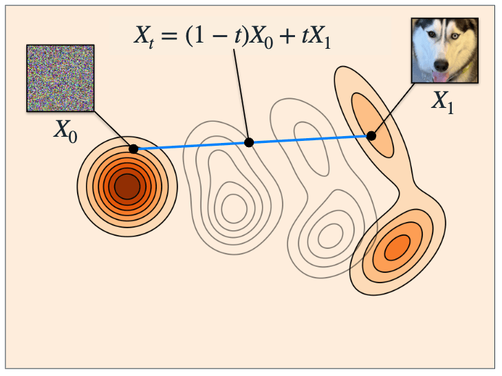
Flow-Matching
Easy to generate.
(Sample noisy interactions.)
Many manipulation trajectories and contact points
combinations are valid, but not all are useful.
Flow-Matching
We cannot
sample from this!
We know how to
sample from this!
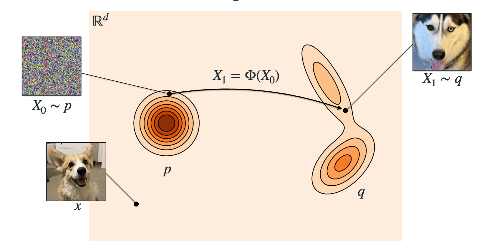
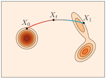
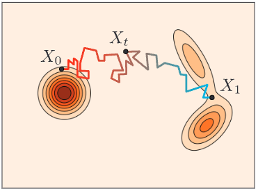
Flow-matching generates new samples from noise by learning a velocity field and integrating it.
Flow-Matching
\(\Phi(^0\mathcal{T})\)
Flow Matching for Contact Modeling
We can learn contacts and manipulation trajectories with "vanilla" flow matching.
-
State space: \(B\)-robot trajectories of \(H\) steps, s.t.,
\[\mathcal{T} \in \mathbb{R}^{B \times H \times 2}\] -
Generation: learn velocity field \(u^\theta_t(\mathcal{T})\) from data, generate new trajectories by
- Sampling \(^0\mathcal{T} \sim \mathcal{N}(\bm{0}, \bm{I})\)
- Integrating: \(^{t+\Delta t}\mathcal{T} \gets ^t\mathcal{T} + u_t^\theta( ^t\mathcal{T}) \cdot \Delta t\)
Flow-Matching
\(\Phi(^0\mathcal{T})\)
Flow Matching for Contact Modeling
We can learn contacts and manipulation trajectories with flow matching.
- Let our state space be the space of \(B\)-robot trajectories of \(H\) steps, s.t.,
\[\mathcal{T} \in \mathbb{R}^{B \times H \times 2}\]
- Once learning a velocity field \(u^\theta_t(\mathcal{T})\) from data, we can generate new trajectories by integrating: \[^{t+\Delta t}\mathcal{T} \gets ^t\mathcal{T} + u_t^\theta( ^t\mathcal{T}) \cdot \Delta t\]
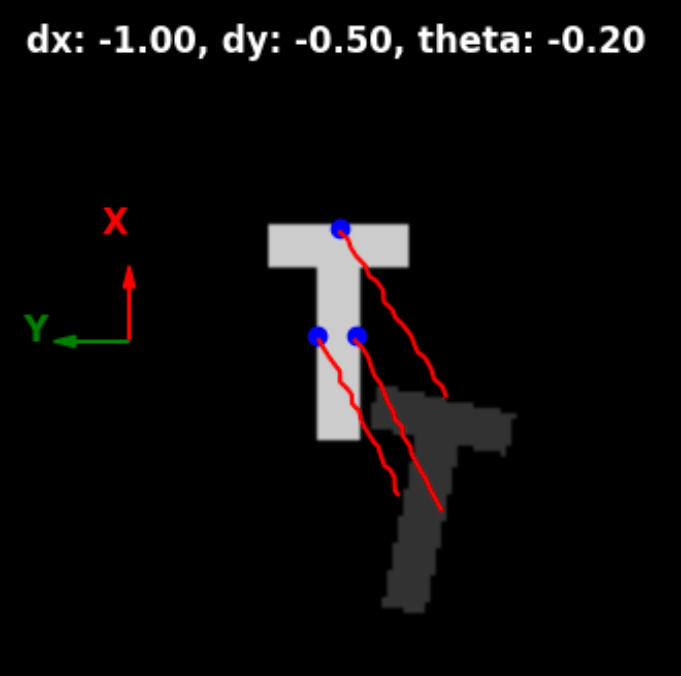
Dataset of \(\langle O, T, \mathcal{K}, \mathcal{T} \rangle\)
Initial Contact
Points
Manipulation
Trajectories
Transform
Observation
Flow Matching for Contact Modeling
We can learn contacts and manipulation trajectories with flow matching.
- Let our state space be the space of \(B\)-robot trajectories of \(H\) steps, s.t.,
\[\mathcal{T} \in \mathbb{R}^{B \times H \times 2}\]
- Once learning a velocity field \(u^\theta_t(\mathcal{T})\) from data, we can generate new trajectories by integrating: \[^{t+\Delta t}\mathcal{T} \gets ^t\mathcal{T} + u_t^\theta( ^t\mathcal{T}) \cdot \Delta t\]
Continuous flow matching for contact modeling.
Continuous flow matching for contact modeling.
Continuous flow-matching was unstable.
Flow Matching for Contact Modeling
Solution:
Split the representation, but generate concurrently.
Continuous flow matching.
Contact Points
\[\mathcal{K} \in \mathbb{R}^{B \times 2}\]
Manipulation Trajectories
\[\mathcal{T} \in \mathbb{R}^{B \times H \times 2}\]
(always rooted at the origin)
Learn two velocity fields, \(u^{\theta}_{\mathcal{K},t}( ^t\mathcal{K})\) and \(u^{\theta}_{\mathcal{T},t}( ^t\mathcal{T})\), and concurrently generate both contact points and manipulation trajectories:
\[^{t+\Delta t}\mathcal{K} \gets ^t\mathcal{K} + u_{\mathcal{K},t}^\theta( ^t\mathcal{K}) \cdot \Delta t\] \[^{t+\Delta t}\mathcal{T} \gets ^t\mathcal{T} + u_{\mathcal{T},t}^\theta( ^t\mathcal{T}) \cdot \Delta t\]
Continuous-Continuous.
Continuous flow-matching co-generation was better, but still unstable.
Flow Matching for Contact Modeling
We can learn contacts and manipulation trajectories with "vanilla" flow matching.
-
State space: \(B\)-robot trajectories of \(H\) steps, s.t.,
\[\mathcal{T} \in \mathbb{R}^{B \times H \times 2}\] -
Generation: learn velocity field \(u^\theta_t(\mathcal{T})\) from data, generate new trajectories by
- Sampling \(^0\mathcal{T} \sim \mathcal{N}(\bm{0}, \bm{I})\)
- Integrating: \(^{t+\Delta t}\mathcal{T} \gets ^t\mathcal{T} + u_t^\theta( ^t\mathcal{T}) \cdot \Delta t\)
Flow-Matching
\(\Phi(^0\mathcal{T})\)
This was not very stable.
We fundamentally have two decisions to make:
- Where to make contact
- How to move.
Flow Matching Co-Generation for Contact Modeling
We fundamentally have two decisions to make:
- Where to make contact
- How to move.
We fundamentally have two decisions to make here:
- Where to make contact
- How to move.
Flow Matching Co-Generation for Contact Modeling
Noisy
Noisy
Clean
Clean
We fundamentally have two decisions to make here:
- Where to make contact
- How to move.
Flow Matching Co-Generation for Contact Modeling
We fundamentally have two decisions to make here:
- Where to make contact
- How to move.
\(u^\theta_\text{dis}\)
\(u^\phi_\text{cont}\)
Flow Matching Co-Generation for Contact Modeling
Generate continuous manipulation trajectories.
We fundamentally have two decisions to make here:
- Where to make contact
- How to move.
\(u^\theta_\text{dis}\)
\(u^\phi_\text{cont}\)
Tie contact points to the
discrete observation-space.
Generate continuous manipulation trajectories.
Flow Matching Co-Generation for Contact Modeling
Contact Point Generation
We can pose this as a discrete problem, asking
which pixels in our image observation should be used for contact points?
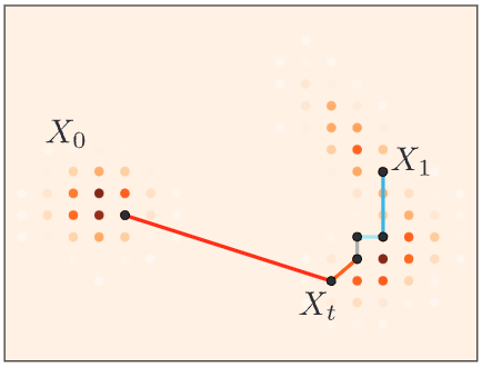
Discrete Flow Matching
Flow
Diffusion
Discrete Flow
Discrete Flow Matching
Let's look at this 2D state space for example:
- State space of token sequences \(\mathcal{S} = \mathscr{T}^d\).
- In our case \(d=2\), and a state is \(x = (x^1, x^2)\).
As before, we require two components:
- A velocity field \(u_t(y,x)\), and
- An initial value \(X_0\).
Getting an initial value is easy. We could
- Sample each token uniformly over the vocabulary
- Set all to a "mask" value \(X_0 = (\texttt{[M]}, \texttt{[M]}, \cdots)\)
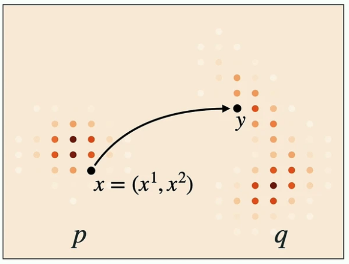
Discrete Flow Matching: Velocity Field
For the velocity field, things are a bit different in the discrete case.
For some state \(x=(x^1, x^2)\), we want
- The probability of \(x^1\) transitioning to \(X^1_1\) should be \(1\), and
- The probability of \(x^2\) transitioning to \(X_1^2\) should be \(1\).
That is, we could define a factorized velocity \(u^i(\cdot, x) = \delta_{X^i_1}\).
Discrete Flow Matching: Interpolation
In continuous flow matching, we asked a model to predict the velocity at some interpolated state \(x_t\).
Given \(X_0\) and \(X_1\), one way to obtain \(X_t\) in the discrete case is to have each element \(X_t^i\) as
- \(X_0^i\) with probability \((1-t)\)
- \(X_1^i\) with probability \(t\)
Discrete Flow Matching: Training
Similar to the continuous case
- Randomly choose \(X_0\) from the noise distribution \(p_0\) and \(X_1\) from the dataset.
- Sample \(t \sim U(0,1)\).
- Get \(X_t\) from "mixing" interpolation.
- Set target velocity \(u^i(\cdot, x) = \delta_{X^i_1}\).
- Supervise on the loss
\[ \mathcal{L}_\text{dis}:= \mathbb{E}_{t, X_1, X_t} \sum_{i} D_{X_t} \left( \dfrac{1}{1-t} \delta(\cdot, X_1^i), u_t^{\theta, i}(\cdot, X_t) \right) \\ \; \\ \theta^* = \arg \min_\theta \mathcal{L}_\text{dis}\]
Discrete Flow Matching: Generation
In essence, a similar process to the continuous case.
Starting with \(X_t = X_0\):
- Compute velocity (i.e., logits) \(u^\theta_t(\cdot, X_t)\)
- Obtain \(X_{t + \Delta t}\) by sampling from the categorical distribution defined by the logits \(u^\theta_t(\cdot, X_t)\)
Flow Matching Co-Generation for Contact Modeling
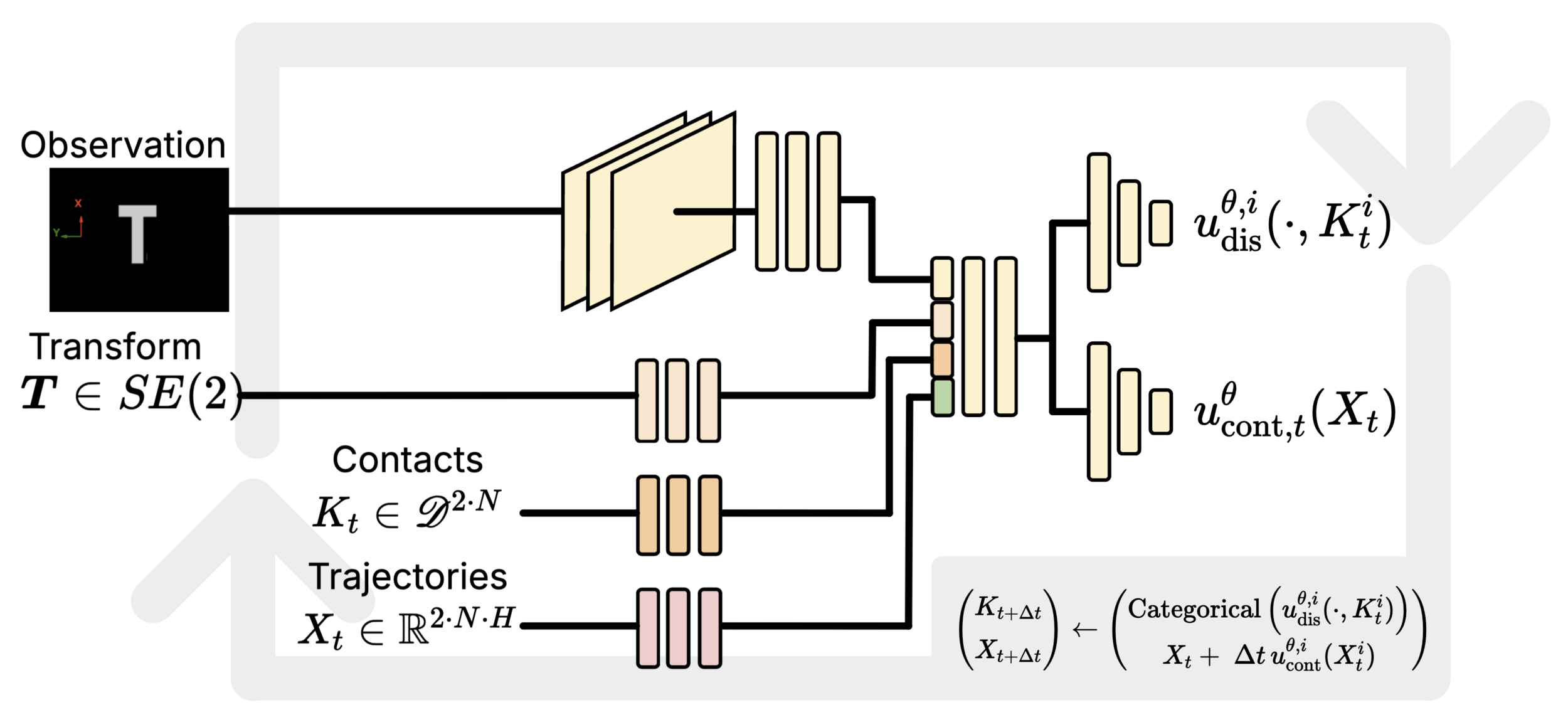
- For flow-matching co-generation [1, 2], operates on two state spaces:
- Discrete contact points: \(K \in \mathscr{D}^{B \times 2}\)
- Continuous trajectories: \(\mathcal{T} \in \mathbb{R}^{B \times H \times 2}\)
- Concurrently learn two velocity fields:
- a continuous velocity field \(u^{\theta}_{\text{cont},t}(^t\mathcal{T})\),
- and "discrete velocity" \(u^{\theta, i}_{\text{dis},t}(\cdot, ^{t\!}K^i)\).
- (Factorized discrete logits.)
- And generate by:
- Sampling \(^0\mathcal{T} \sim \mathcal{N}(\bm{0}, \bm{I})\) and \(^0K := \{(\text{M},\text{M})\}^B\)
- Integrating
\(u^\theta_\text{dis}\)
\(u^\phi_\text{cont}\)
Flow Matching Co-Generation for Contact Modeling
- For flow-matching co-generation [1, 2], operates on two state spaces:
- Discrete contact points: \(K \in \mathscr{D}^{B \times 2}\)
- Continuous trajectories: \(\mathcal{T} \in \mathbb{R}^{B \times H \times 2}\)
- Concurrently learn two velocity fields:
- a continuous velocity field \(u^{\theta}_{\text{cont},t}(^t\mathcal{T})\),
- and "discrete velocity" \(u^{\theta, i}_{\text{dis},t}(\cdot, ^{t\!}K^i)\).
- (Factorized discrete logits.)
- And generate by:
- Sampling \(^0\mathcal{T} \sim \mathcal{N}(\bm{0}, \bm{I})\) and \(^0K := \{(\text{M},\text{M})\}^B\)
- Integrating
Flow Matching Co-Generation for Contact Modeling
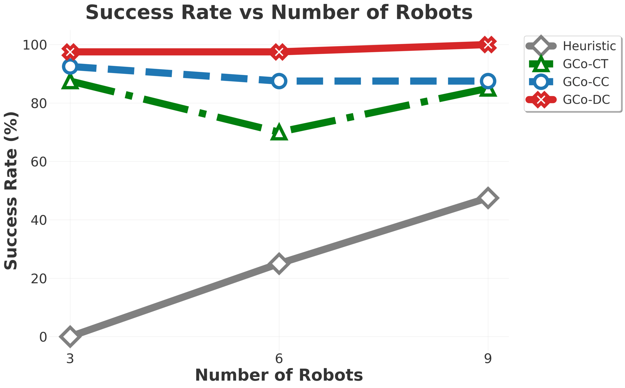
- Discrete-contnuous flow-matching proved to be more robust than alternatives.
- Continuous-continuous flow matching followed,
- Continuous "naive" flow matching was least stable.

Observation
Transform
Contacts
\(K_t \in \mathscr{D}^{2\cdot N}\)
Trajectories
\(X_t \in \mathbb{R}^{2\cdot N \cdot H} \)
Flow Matching Co-Generation for Contact Modeling
Flow Matching Co-Generation for Contact Modeling
- For flow-matching co-generation [1, 2], operates on two state spaces:
- Discrete contact points: \(K \in \mathscr{D}^{B \times 2}\)
- Continuous trajectories: \(\mathcal{T} \in \mathbb{R}^{B \times H \times 2}\)
- Concurrently learn two velocity fields:
- a continuous velocity field \(u^{\theta}_{\text{cont},t}(^t\mathcal{T})\),
- and "discrete velocity" \(u^{\theta, i}_{\text{dis},t}(\cdot, ^{t\!}K^i)\).
- (Factorized discrete logits.)
- And generate by:
- Sampling \(^0\mathcal{T} \sim \mathcal{N}(\bm{0}, \bm{I})\) and \(^0K := \{(\text{M},\text{M})\}^B\)
- Integrating
The models flexibly select number of robots, given a budget.
Flow Matching Co-Generation for Contact Modeling
Let's assume, for a moment, that we know how to plan for robots and objects.
Planning and Learning For Collaboration
- Observe objects.
- Plan object transformations.
- Generate manipulation interactions.
- Plan robot trajectories.
- Execute and repeat.
Plan motions
to contact points
Learn physical
interactions
Plan motions
for objects
Let's assume, for a moment, that we know how to plan for robots and objects.
Planning and Learning For Collaboration
Planning and Learning For Collaboration
Plan motions
to contact points
Learn physical
interactions
Plan motions
for objects
- Observe objects.
- Plan object transformations.
- Generate manipulation interactions.
- Plan robot trajectories.
- Execute and repeat.
Let's assume, for a moment, that we know how to plan for robots and objects.
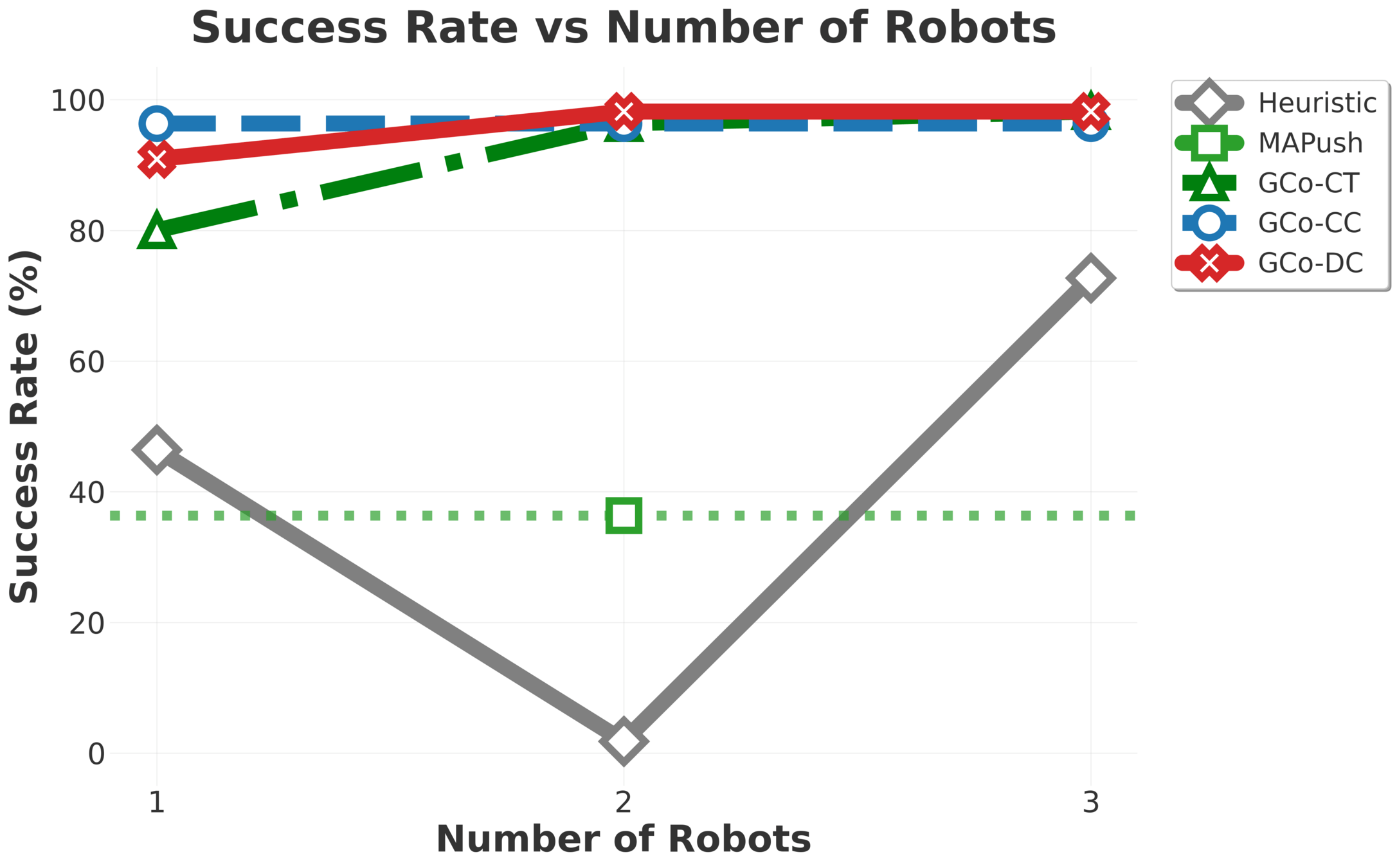
Collaborative Manipulation - Exprimental Evaluation
\(\text{GC}\scriptsize{\text{O}}\) composes per-object models, scaling to nine robots and five objects, including cases where objects outnumber robots.
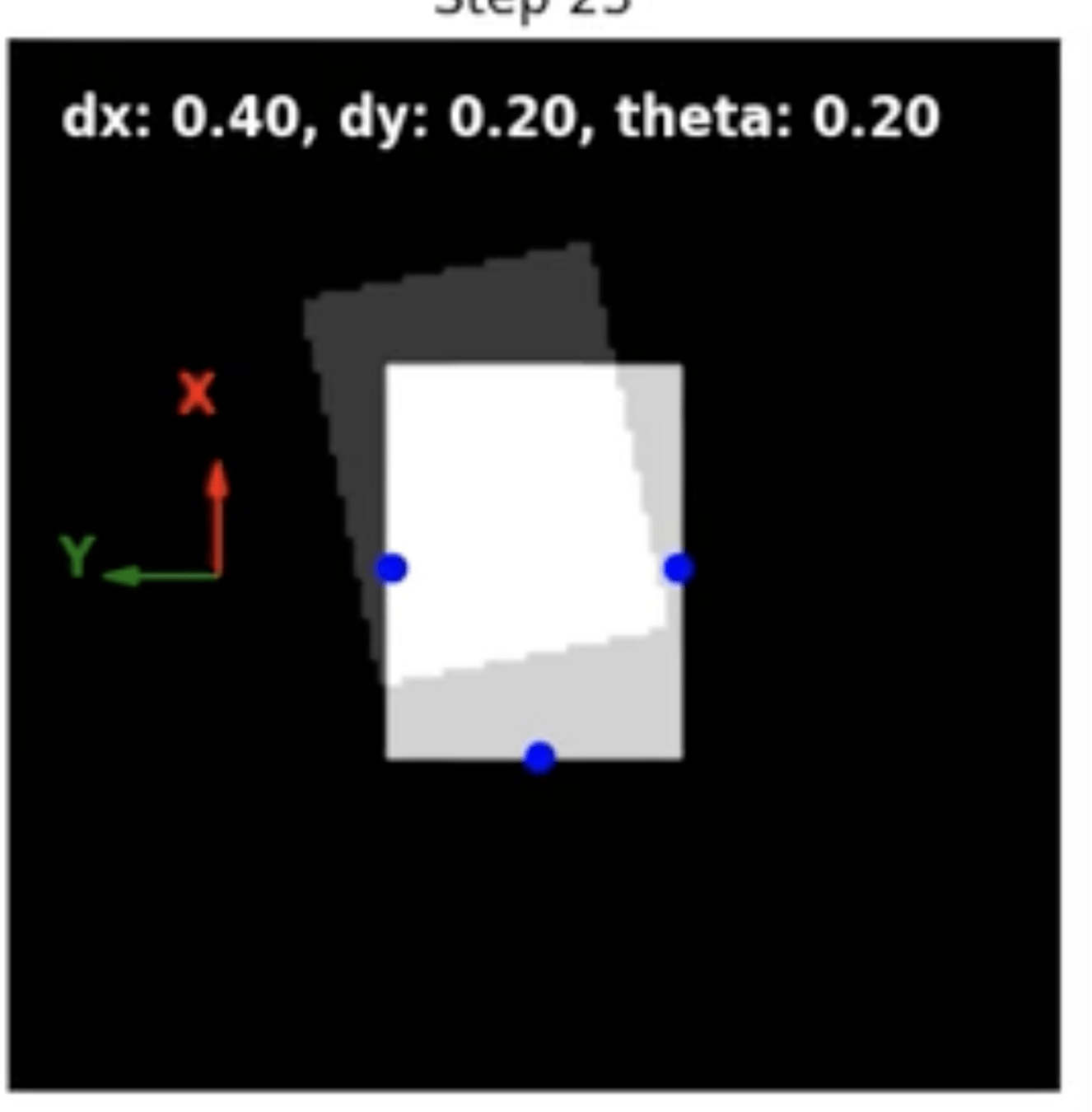
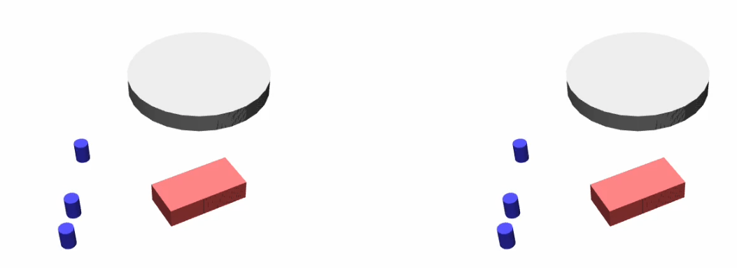
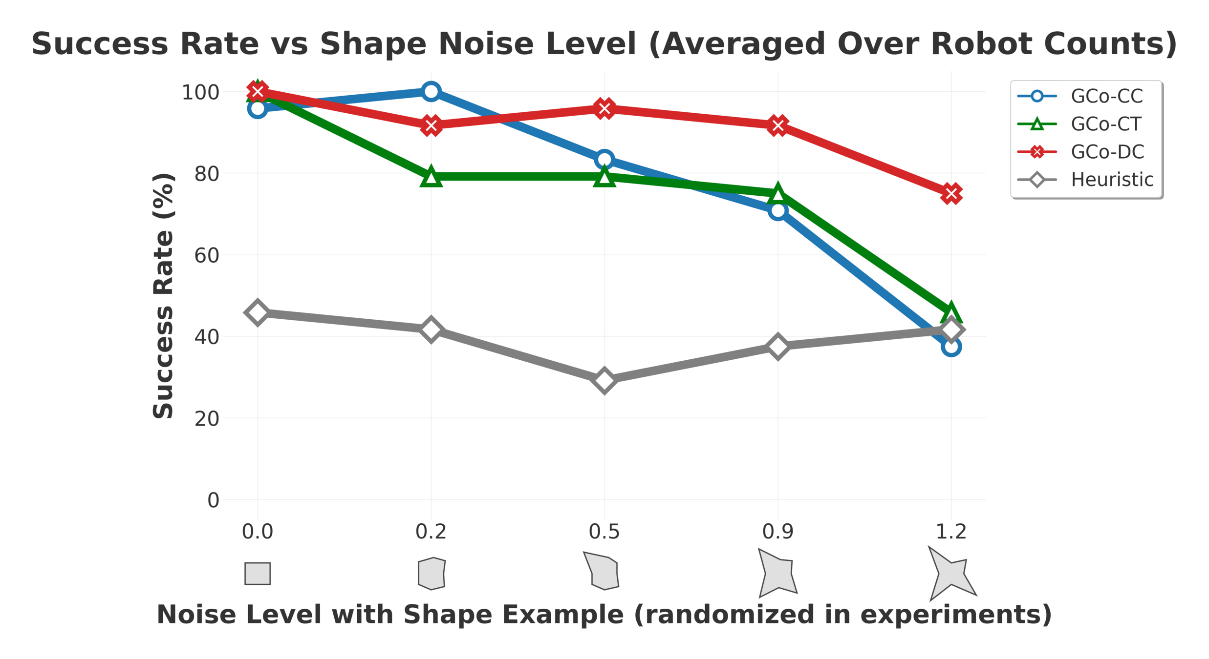
Collaborative Manipulation - Stress Testing
Despite being trained only on rectangles and circles, the models handle arbitrary polygons thanks to the flexibility in the observation medium.
In distribution.
Out of distribution.
Collaborative Manipulation - Brief Results
Gradually increasing test difficulty.
Agenda
- We'll start by looking at learning manipulation interactions,
- Continue to our multi-robot planning algorithm \(\text{G}\scriptsize{\text{SPI}}\),
Plan motions
to contact points
Learn physical
interactions
Plan motions
for objects
Planning and Learning For Collaboration
Anonymous Multi-Robot Motion Planning
Object- and robot-planning fall under the same algorithmic umbrella.
- Given a set of goal configurations,
- Compute motions for all entities to
reach them.- Assignment is not fixed.
Plan compositions of short actions
Anonymous Multi-Robot Motion Planning
Object- and robot-planning fall under the same algorithmic umbrella.
- Given a set of goal configurations,
- Compute motions for all entities to
reach them.- Assignment is not fixed.
Plan compositions of short actions
Problem Formulation
Go from here to there (it does not matter who goes where).
Anonymous Multi-Robot Motion Planning
Minimizing
- Sum of costs or makespan (the time taken for all robots to arrive at goals).
- The computation time (overall or time-to-next-motion (if applicable)).
Anonymous motion planning has been explored in the Multi-Agent Path Finding (MAPF) community.
Some Background: TSWAP
kei18.github.io
Most algorithms, like TSWAP, operate on regular grids.
But we want to operate in "continuous" spaces.
We take an intermediate approach, with motion-primitives.
Key ideas: swap goals between robots when it benefits the system.
Anonymous MAPF, traditionally, is solved on regular grids.
Some Background: Motion Primitives
Regular grid.
Motion primitives.
Swapping goals between robots when their next-best steps conflict with each other works... sometimes.
Other times it leads to deadlocks.
Naive Goal Swapping with Motion Primitives
Some Background: PIBT
An extremely scalable turn-by-turn procedure for labeled MAPF.
In a nutshell, high priority robots can push away lower priority ones.
Some Background: PIBT
An extremely scalable turn-by-turn procedure for labeled MAPF.
A single robot (loosely) operates as follows:
- Initialize a random priority \(\in [0,1]\) (without repetition with others).
Then, in the order of priorities:
- Choose next step in direction of goal.
- If step is occupied:
- The blocking robot inherits the priority of the acting robot.
- The blocking robot attempts to move away in a way that does not collide with the acting robot.
- Recursively called on blocking robots until a safe motion is found.
This is not only a continuous-space issue, actually. PIBT only guarantees reachability and not remaining at goals.
PIBT with Motion Primitives
Works... sometimes.
Anonymous Multi-Robot Motion Planning
What we want
Livelocks
Deadlocks
What we get
(from naively applying existing AMAPF ideas)
To mitigate these issues, we developed the "\(\text{G\scriptsize SPI}\)" algorithm, a "continuous-space" hybrid adaptation of PIBT with gaol-swapping inpired by TSWAP and C-UNAV.
Anonymous Multi-Robot Motion Planning
PIBT
+ Goal Swapping
= \(\text{G\scriptsize SPI}\) (Goal Swapping with Priority Inheritance)
Suffers from livelocks
Suffers from deadlocks
In a nutshell:
Setup:
- Robots \(R^i\) assigned goals \(g^i\), and priorities \(\prec\) initialized.
Loop:
- For \(R^i, R^j\), if
- Swapping goals benefits higher priority \(R^i\) (\(R^i \prec R^j\)), and swapping goals benefits overall system cost:
- Swap goals and priorities.
- Swapping goals benefits higher priority \(R^i\) (\(R^i \prec R^j\)), and swapping goals benefits overall system cost:
- Each robot proposes best-next motion primitive.
- Robots \(R^i \prec R^j\) recursively reserve volumes.
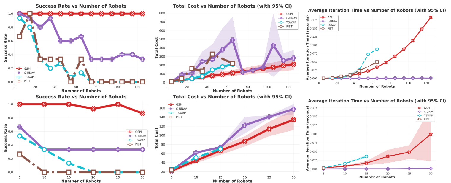
\(\text{G\scriptsize SPI}\)
\(\text{G{\scriptsize SPI}}\)
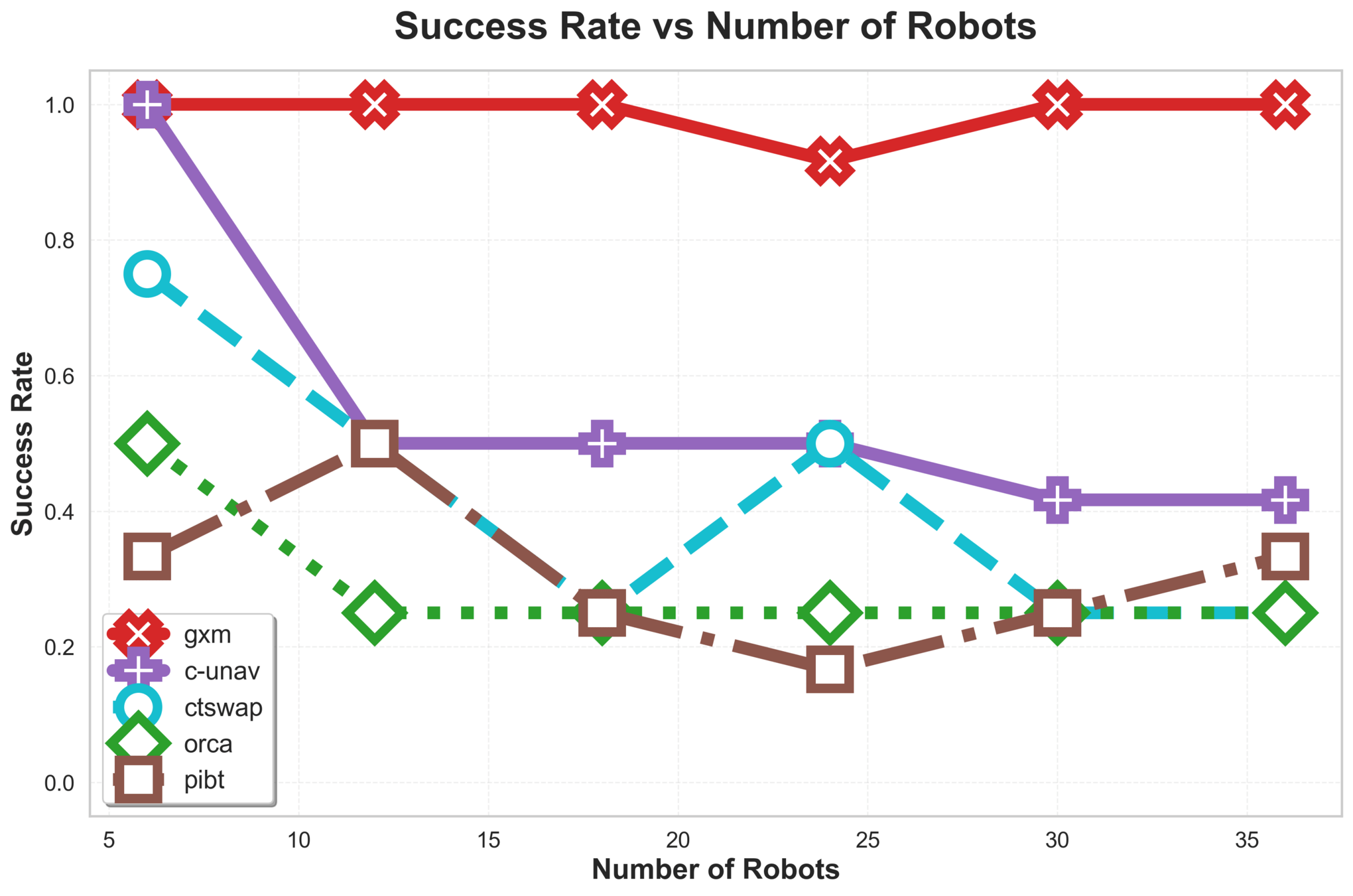
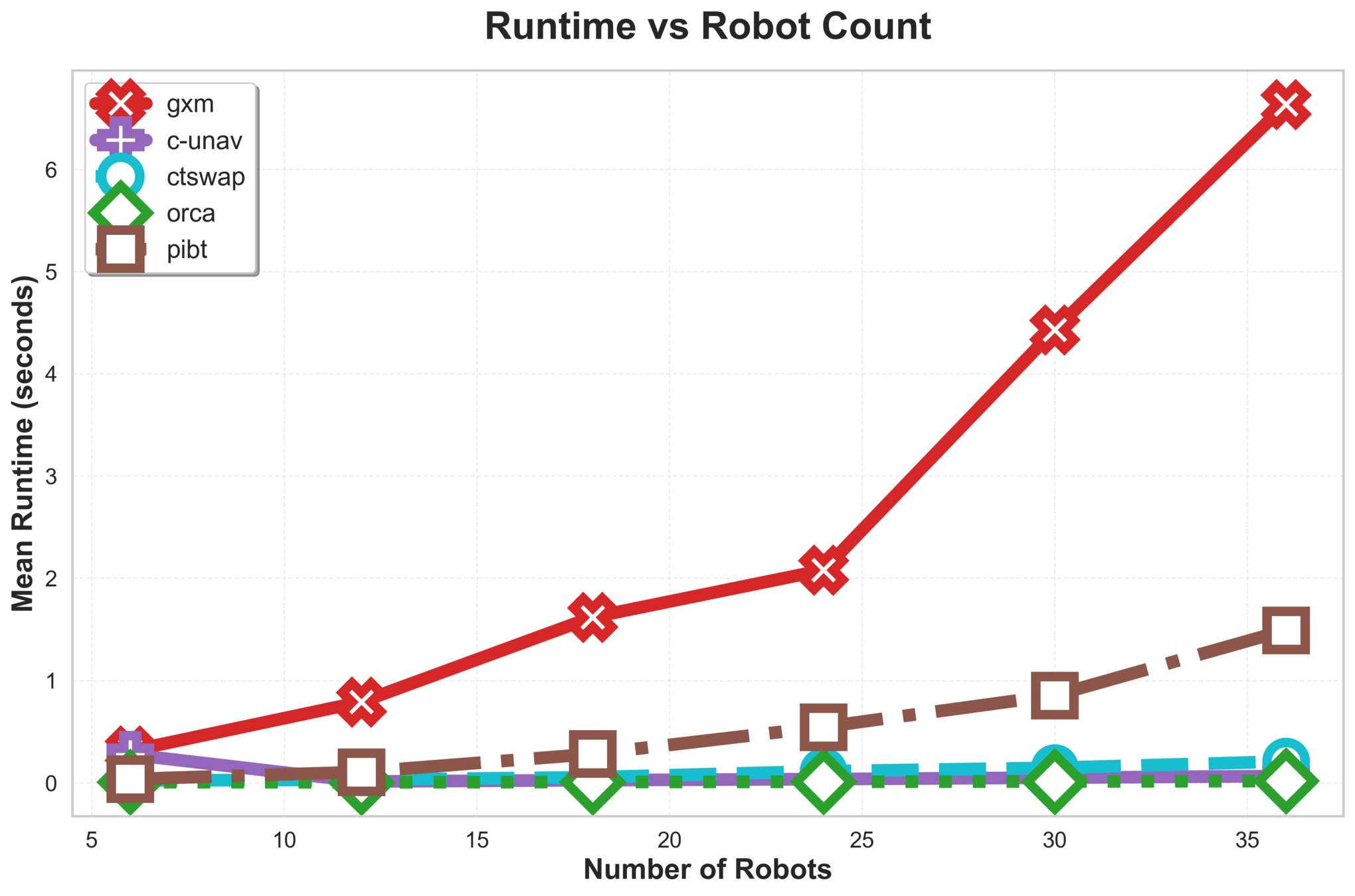
\(\text{{G\scriptsize SPI}}\) is efficient and scales to 300 robots in our experiments.
Straight lines are the result of effective goal swapping.
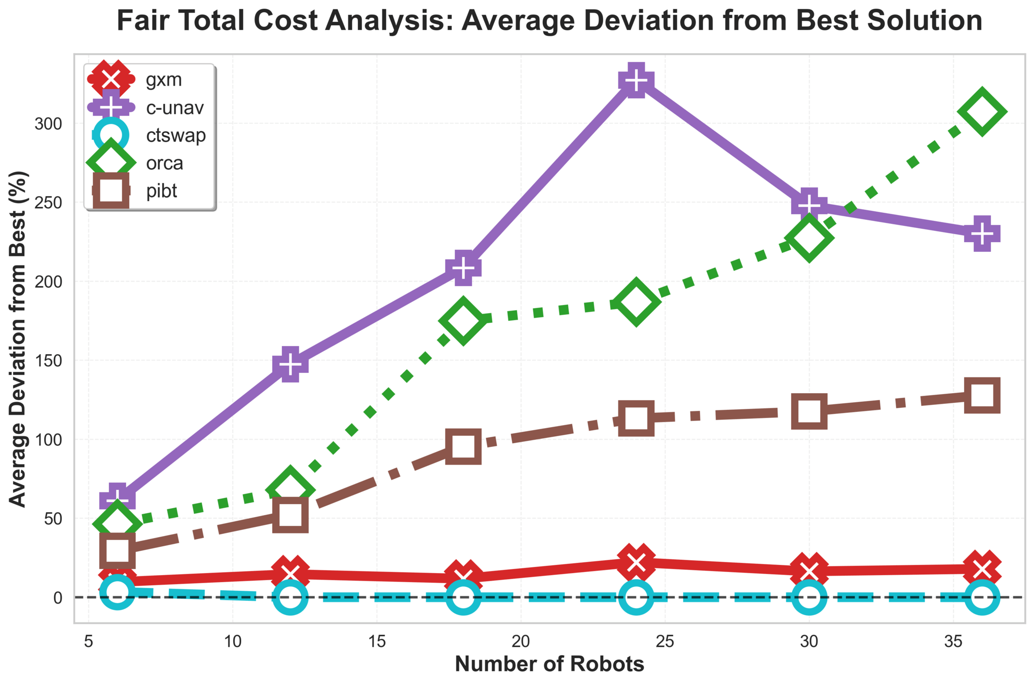
\(\text{G{\scriptsize SPI}}\) Analysis
\(\text{{G\scriptsize SPI}}\) handles stress tests that often break algorithms:
- Extremely tight spaces and "following" concurrent movements.
\(\text{G{\scriptsize SPI}}\) Analysis
Some results
\(\text{G{\scriptsize SPI}}\) Analysis
Results
\(\text{G{\scriptsize SPI}}\) Analysis
C-UNAV / ORCA
Failure cases for baselines
PIBT
TSWAP
One Step-Manipulation
Move robots, manipulate a single object.
Composing Manipulation Policies with Planning
- Observe objects,
- \(\text{G{\scriptsize SPI}}(\text{Objects})\),
- Generate manipulation interaction,
- \(\text{G{\scriptsize SPI}}(\text{Robots})\),
- execute, repeat.
Agenda
- We'll start by looking at learning manipulation interactions,
- Continue to our multi-robot planning algorithm \(\text{G}\scriptsize{\text{SPI}}\),
Plan motions
to contact points
Learn physical
interactions
Plan motions
for objects
Planning and Learning For Collaboration
Agenda
- We'll start by looking at learning manipulation interactions,
- Continue to our multi-robot planning algorithm \(\text{G}\scriptsize{\text{SPI}}\),
Plan motions
to contact points
Learn physical
interactions
Plan motions
for objects
Planning and Learning For Collaboration